Change of Variables and the Jacobian
May 18, 2020
In single-variable calculus, we can integrate functions of the form
\[g'(x)f(g(x))\]
by 'rephrasing' the entire integral as an integral of \(g(x)\) instead of an integral of \(x\). This is known as substitution. For example, consider the following integral:
\[\int x e^{x^2} dx\]
Integrating this function as it currently is is painfully annoying, and so Leibniz, one of the fathers of calculus, came up with a way to simplify this integral. The first step in doing so is to notice that
\(x\) can be represented as a derivative of \(x^2\). More precisely, if we let \(u=x^2\), then
\[\frac{du}{dx} = 2 x\]
\[du = 2 xdx\]
Notice how this is very similar to the \(xdx\) we had in our original integrand, except it has a coefficient of \(2\). It follows, then, that in order for \(du\) to equal \(xdx\), we must divide it by two,
\[xdx = \frac{1}{2} du\]
We can now substitute the variables in our original integral with the new ones,
\[\int x e^{x^2} dx = \frac{1}{2} \int e^u du\]
making the integral trivially easy to solve:
\[ \frac{1}{2} \int e^u du = \frac{e^u}{2} + C = \frac{e^{x^2}}{2} + C\]
Now, if we want to use an analogous process for functions of several variables, how would we do that?
Change of Variables
Consider the double integral
\[\iint_D 3x\sin(6x+7y) - y \sin(6x+7y) dxdy\]
While this integral isn't impossible to solve, we can greatly simplify the process by employing a change of variables. First, we define the transformation
\[T: D \rightarrow D^*\]
such that
\[T(x, y) = (u, v)\]
where \(u=3x-y\) and \(v=6x+7y\). This transformation transforms the domain \(D\) in \(xy\) space to a domain \(D^*\) in \(uv\) space. If \(D\) was the unit square \([0, 1]\times[0, 1]\), for example, the transformation \(T\) would "stretch" or "squeeze" the unit square into a parallelogram with a different area. Keep this notion in mind, as it will be important in the next step (later in the post I give examples of other transformations).
Now that we have our substitutions for \(x\) and \(y\), we can just replace them with our new variables and integrate over the new domain \(D^*\)...
\[\iint_D 3x\sin(6x+7y) - y \sin(6x+7y) dxdy \stackrel{?}{=} \iint_{D^*} u \sin v dudv\]
... right?
Well, not exactly. The problem is that the infinitesimal area \(dudv\) is different than the infinitesimal area \(dxdy\) precisely because the area of the domain as a whole changes after being transformed. In order to fix this, wouldn't it really cool if we had a tool for determining by how much the infinitesimal area \(dxdy\) is scaled when transformed? That's where the Jacobian comes in.
Jacobian Matrices
The Jacobian matrix of a transformation, or, more precisely, its determinant, tells us exactly by how much the transformation scales the infinitesimal area. The Jacobian matrix of the transformation \(T\) (as defined above) looks like this:
\[\left| \frac{\partial (u, v)}{\partial (x, y)}\right| = \left| \begin{matrix} \frac{\partial u}{\partial x} & \frac{\partial u}{\partial y} \\ \frac{\partial v}{\partial x} & \frac{\partial v}{\partial y} \end{matrix} \right|\]
Let's think about why the determinant of such a matrix might give us the factor by which the area is scaled.
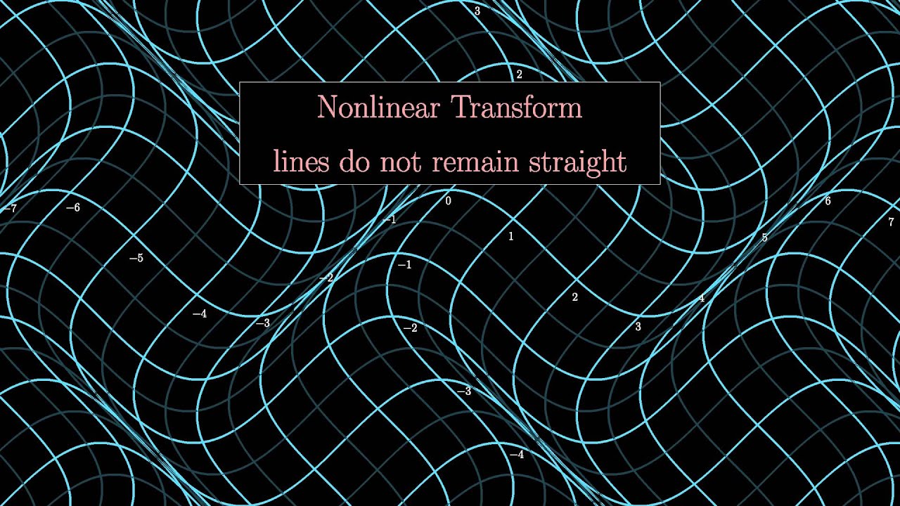
In the same way that a smooth, continuous function looks more and more like a straight line the more you 'zoom in' on a point, a smooth, continuous transformation, looks more and more like a linear transformation the more you zoom in. Below is a perfect example: a non-linear transformation that warps space, but it's not difficult to imagine that as you 'zoom in', which really just means paying attention only to points around some given point, one could locally approximate this transformation with a linear one.
Now, we can take advantage of this fact by considering the infinitesimal area dxdy at some point \((x_0, y_0)\):
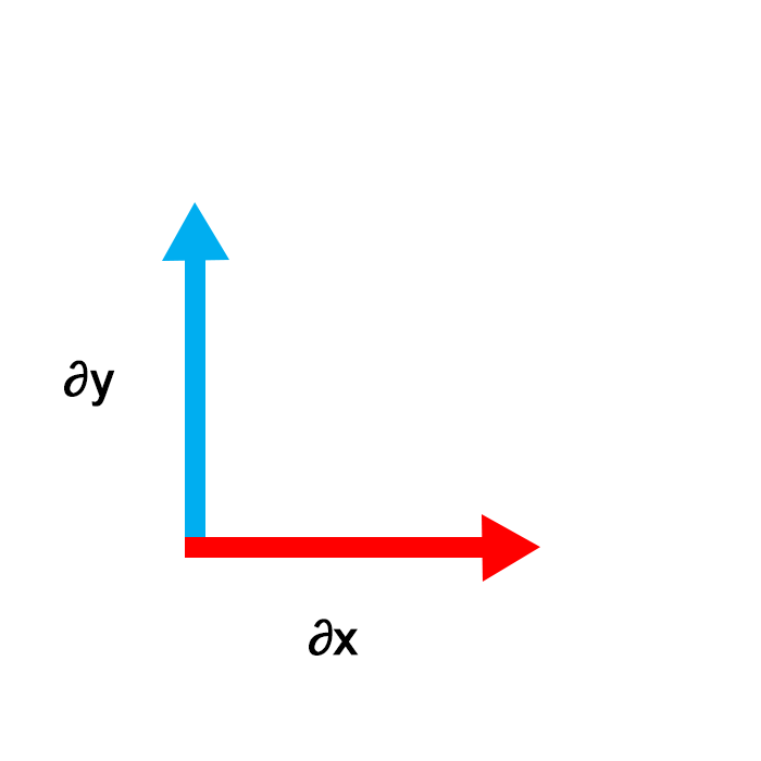
If we think of the two columns in the Jacobian matrix as transformations of the basis vectors,
\[T_x = \left[ \begin{matrix} \frac{\partial u}{\partial x} \\ \frac{\partial v}{\partial x}\end{matrix}\right], \ \ \ \ T_y = \left[ \begin{matrix} \frac{\partial u}{\partial y} \\ \frac{\partial v}{\partial y}\end{matrix}\right]\]
then \(T_x\) tells us how much \(\partial x\) is scaled and \(T_y\) tells us how much \(\partial y\) is scaled.
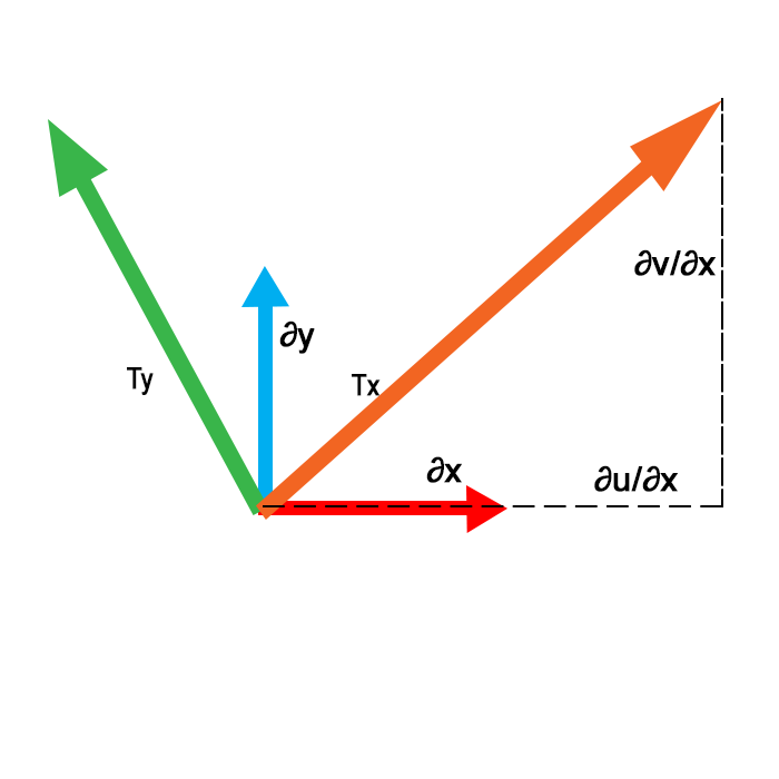
As the diagram shows, \(\partial u/\partial x\) tells us how much an infinitesimal step in the \(x\) direction is scaled in the \(u\) direction, \(\partial v / \partial x\) tells us how much a step in the \(x\) direction is scaled in the \(v\) direction, and so on.
Taking the determinant of these two vectors (which together form the Jacobian matrix) essentially gives us the ratio of area of parallelogram these two new vectors form to the area of the paralleogram the vectors in \(xy\) space form, which tells us exactly how much it's scaled.
Multiplying this by \(dxdy\) in the integrand gives us the 'correctly sized' areas which we integrate. And so, the 'scaled' integral actually looks like this,
\(\iint_D 3x\sin(6x+7y) - y \sin(6x+7y) dxdy = \iint_{D^*} u \sin v \left|\frac{\partial (u, v)}{\partial (x, y)}\right| dudv\) \(= \iint_{D^*} u \sin v \left| \begin{matrix} \frac{\partial u}{\partial x} & \frac{\partial u}{\partial y} \\ \frac{\partial v}{\partial x} & \frac{\partial v}{\partial y} \end{matrix} \right| dudv\)
\(= \iint_{D^*} u \sin v \left| \begin{matrix} 3 & -1 \\ 6 & 7 \end{matrix} \right| dudv\) \(= 27 \iint_{D^*} u \sin v dudv\)
Applications
The most common application of the change of variables method is most likely converting between different coordinate systems. If we want to evaluate the integral
\[\iint_D f(x, y)dxdy\]
in polar coordinates, first we define the transformation, \(x=r\cos\theta, \ \ \ \ y= r\sin\theta\)
then we set up and evaluate the Jacobian
\[\left| \frac{\partial (x, y)}{\partial (r, \theta)}\right| = \left| \begin{matrix} \cos\theta & -sin\theta \\ \sin\theta & r\cos\theta \end{matrix} \right| = rcos^2\theta + rsin^2\theta = r\]
And finally, we can complete the change of variables:
\[\iint_D f(x, y)dxdy = \iint_{D^*} f(r\cos\theta, r\sin\theta) \left| \frac{\partial (x, y)}{\partial (r, \theta)}\right| dr d\theta = \iint_{D^*} f(r\cos\theta, r\sin\theta) r dr d\theta\]
And that's how you can use the Jacobian and the change of variables method to greatly simplify solving all sorts of integrals. I hope you found this helpful!